Predictions with Linear Regression

This is my first attempt at building a Linear Regression model using Snowflake's Snowpark. I built two different Linear Regression models.

One using Snowflake's Snowpark and the other using Python's sciki-learn model.

I then compare the predicted results based on the results from the model that I built in Python.

Overview

The objective is to predict inflation based on historical data from Snowflake's data cloud. We will process data with Snowpark, develop a simple ML model and create a Python User Defined Function (UDF) in Snowflake.

Getting The Data

We shall get the data from the Snowflake marketplace.  FINANCIAL__ECONOMIC_ESSENTIALS. The table we will be using is the Financial_Fred_Timeseries data.

Create a New Database

Once we have received the data source, we need to create a database that will store our User Defined Function (UDF). We will create a database with the name SUMMIT_HOL

-- Setup database, need to be logged in as accountadmin role
-- Set role and warehouse (compute)
USE ROLE accountadmin;
USE WAREHOUSE compute_wh;

--Create database and stage for the Snowpark Python UDF
CREATE DATABASE IF NOT EXISTS summit_hol;
USE DATABASE summit_hol;
CREATE STAGE IF NOT EXISTS udf_stage;

Explore Data with Jupyter Notebook

I first need to initialize Notebook, import libraries and create Snowflake connection

Creating Features for ML Training

We want to predict the Personal consumption price index (PCE) . So we will need to create a Pandas dataframe that can be used for training the model with the scikit-learn Linear Regression model. The .to_pandas() function - pushes the query to Snowflake and return the results as a Padas dataframe. 

In the above example, we set up the Data Frame by creating this SQL statement using data frame style programming. When you run this, you get the same data back - now it's done through data frames. 

Train the Linear Regression Model

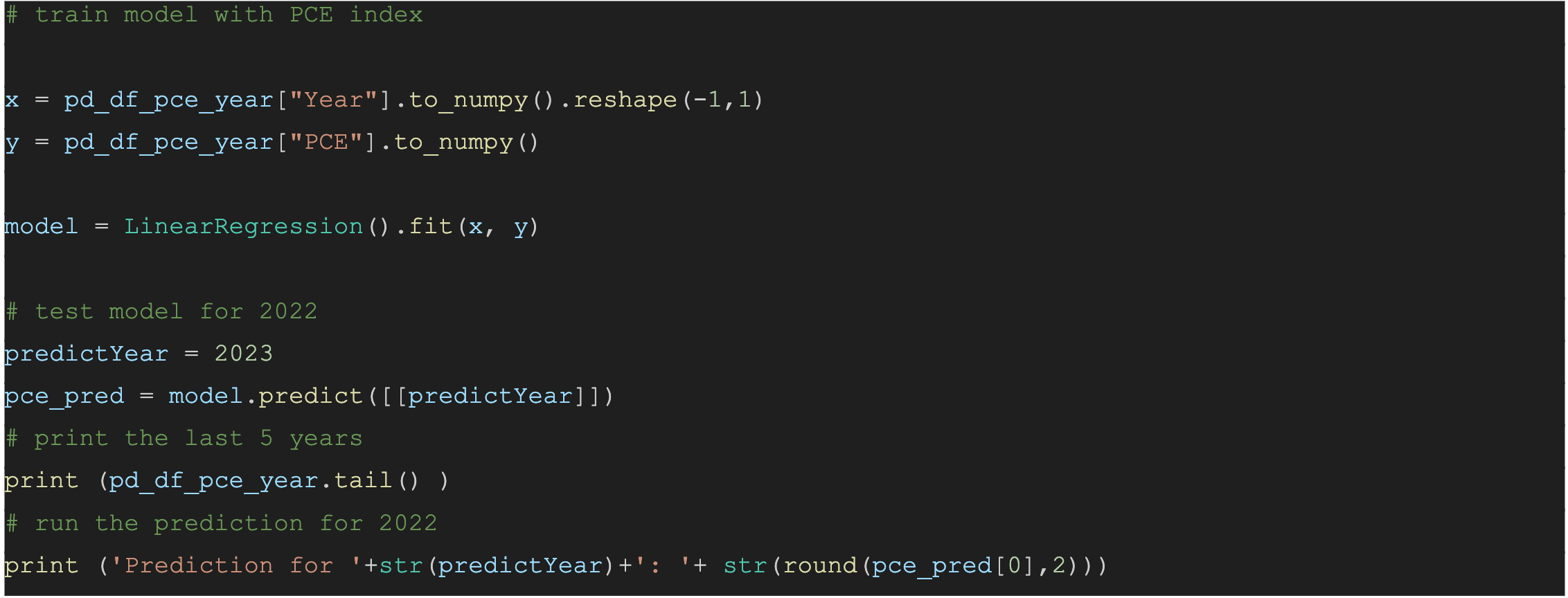
Once we have created the features, we can train the model. We will transform the Pandas dataframe with the features to arrays using the NumPy library. Once trained we can display a prediction. 

Actual values for 2023 are 119.01 - and the predicted values were 113.47

Creating a User Defined Function within Snowflake to do the score there

Here, we are deploying this UDF into Snowflake and it does that inside the udf_stage. We specify which packages are needed to run this function. 

Test the UDF using a SQL command in Python

We can then leverage this function in future SQL Series. At this point, we are done building a simple model using Snowpark. In the section below, I build a separate Linear Regression in Python with the same dataset mentioned above.

I built the following Linear Regression model using scikit-learn and then compared the results of the 2 models.

Step 1: Import the necessary Libraries and read the dataset.

Step 2: Prepare the Dataset

Split the dataset into features X (Year) and target variable y (Value). Basically extracting the independent variable (Year) and the dependent variable (Value) 

Step 3: Split the Dataset

The dataset is split into training and testing sets using scikit-learn’s ‘train_test_split()’ function. 

Step 4: Fitting Linear Regression Model

We create and instance of the Linear Regression model and fit it to the training data using the ‘fit()’ method. We create a linear regression model using ‘LinearRegression’ from ‘scikit-learn’

Create a Linear Regression object 
model=LinearRegression()

Train the model using the training sets
model.fit(X_train, y_train)

Step 5: Making Predictions

We use the trained model to make predictions on both the training and testing sets.The model is trained using the training data (X_train and y_train).

Step 6: Evaluating the Model

We calculate the Root Mean Squared Error (RMSE) for both the training and testing sets to evaluate the performance of the model. Lower RMSE values indicate better model performance.

Mean Absolute Error (MAE): 3.6429708092429847
Mean Squared Error (MSE): 21.783922761054384
Root Mean Squared Error (RMSE): 4.6673250112944125

Step 7: Plot Existing Dataset

Just to visualise what the dataset looks like before we make any predictions.

Step 8: Run the model to predict values for the next 5 years

We can use our trained model to predict the value for the Year 2023.

Predicted value for the year 2023: [111.25635893]

Using the model. lets predict the values for the next 5 years of values starting from 2020.

Year: 2020, Value: 106.28741227408727
Year: 2021, Value: 107.94372782544497
Year: 2022, Value: 109.60004337680266
Year: 2023, Value: 111.25635892816035
Year: 2024, Value: 112.91267447951805
Year: 2025, Value: 114.56899003087574
Year: 2026, Value: 116.22530558223343

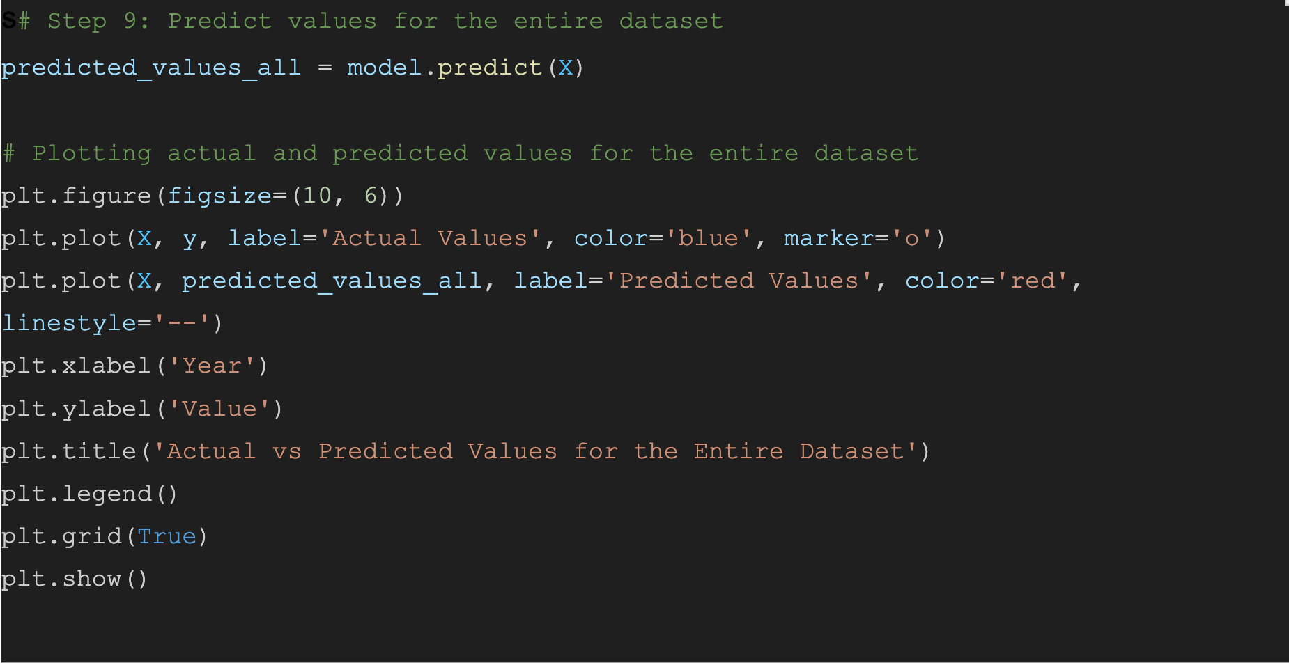
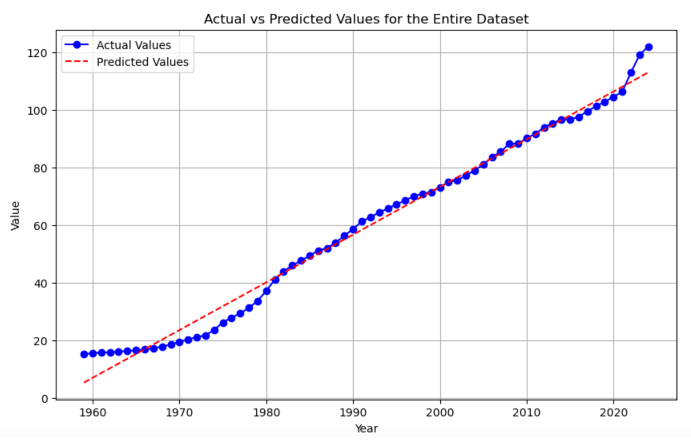
Step 9: Plot Actual & Predicted Values

We can plot both the actual and predicted values for the entire dataset to visualize how well our model fits the data.

Thanks for reading